Daily, Weekly and Yearly seasonalities.

A lot of signals have calendar based seasonalities:

• city noise levels have a daily seasonality: it's busy when people are out and calm at night.
• sales have a weekly seasonality: people buy more on Wednesdays and Saturdays.
• and for yearly seasonality ...you guessed it, seasons.

These seasonalities are hard to define with a simple mathematical function, but most of the time you have a rough idea of their shape. Let's see how you can create them with mockseries !

Daily seasonality

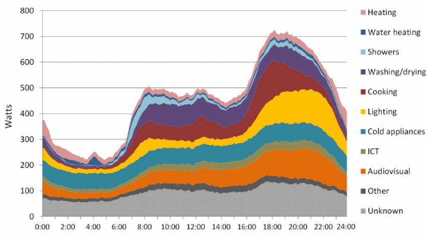
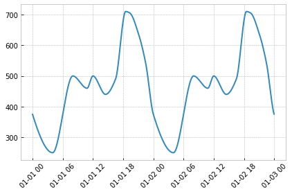
Let's look at the hourly energy consumption per household. It's definitely cyclic: you consume less when you're sleeping, and there are pics corresponding to breakfast, lunch and dinner: things that happen everyday. To generate a similar signal in mockseries, we just need to identify a few constraint points. A constraint is a time and its associated value.
An algorithm will generate a realistic curve that respects the constraints.
Times are expressed as timedeltas from the start of the period, so for DailySeasonality, timedeltas should be between 0h 0min 0 sec and 23h 59min 59.999sec.

# plotting utilities for the whole tutorial

import matplotlib.pyplot as plt

DEFAULT_SIZE_PLOT = plt.rcParamsDefault["figure.figsize"]

LARGE_SIZE_PLOT = (20,7)

from datetime import datetime, timedelta

from mockseries.seasonality import DailySeasonality

# create the daily seasonality signal

constraints = {

timedelta(hours=0): 375,

timedelta(hours=4): 250,

timedelta(hours=8): 500,

timedelta(hours=10, minutes=50): 460,

timedelta(hours=12): 500,

timedelta(hours=14, minutes=30): 440,

timedelta(hours=16, minutes=30): 490,

timedelta(hours=18, minutes=30): 710,

timedelta(hours=18, minutes=30): 710,

timedelta(hours=19, minutes=20): 705,

timedelta(hours=21): 640,

timedelta(hours=22, minutes=30): 540,

}

daily_seasonality = DailySeasonality(constraints)

# quick plotting on 2 days

daily_seasonality.preview_day(num_days=2, start_time=datetime(2021, 1, 1))

That's it ! WeeklySeasonality and YearlySeasonality work the same way, the 3 signals are subclasses of the PeriodSeasonality. But don't leave just yet! We still have important features to explore.

Weekly seasonality - Managing timezone

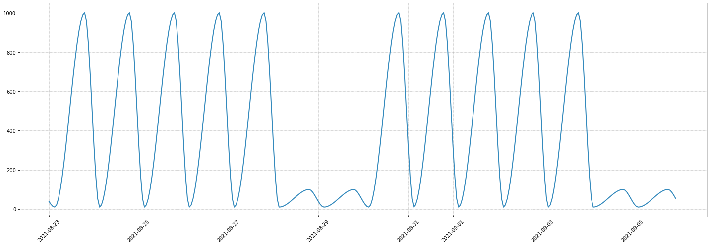
Let's imagine the weekly traffic of an american social network:

• the app has almost no users at night
• the app has many users around 7pm, except on Saturday and Sunday and

Let's use WeeklySeasonality to get this:

plt.rcParams["figure.figsize"] = LARGE_SIZE_PLOT

from mockseries.seasonality import WeeklySeasonality

constraints = {

timedelta(hours=3): 10, ### EARLY MONDAY

timedelta(days=1, hours=3): 10, ### EARLY TUESDAY

timedelta(days=2, hours=3): 10, ### EARLY WEDNESDAY

timedelta(days=3, hours=3): 10, ### EARLY THURSDAY

timedelta(days=4, hours=3): 10, ### EARLY FRIDAY

timedelta(days=5, hours=3): 10, ### EARLY SATURDAY

timedelta(days=6, hours=3): 10, ### EARLY SUNDAY

timedelta(hours=19): 1000, ### MONDAY EVENING

timedelta(days=1, hours=19): 1000, ### TUESDAY EVENING

timedelta(days=2, hours=19): 1000, ### WEDNESDAY EVENING

timedelta(days=3, hours=19): 1000, ### THURSDAY EVENING

timedelta(days=4, hours=19): 1000, ### FRIDAY EVENING

timedelta(days=5, hours=19): 100, ### SATURDAY EVENING

timedelta(days=6, hours=19): 100, ### SUNDAY EVENING

}

weekly_seasonality = WeeklySeasonality(constraints)

weekly_seasonality.preview_week(num_weeks=2, start_time=datetime(2021, 8, 23))

Looks nice, but there's one problem. The social network is american, straight from the Silicon Valley ! All times were given with PDT timezone in mind.
It's easy to do this in mockseries: just pass the UTC offset of the timezone. For instance: PDT is UTC-7: just pass an utc_offset of `-7 hours.

from mockseries.utils.dates import datetime_range

from mockseries.utils.plot import plot_timeseries

PDT_OFFSET = timedelta(hours=-7)

weekly_seasonality = WeeklySeasonality(constraints)

weekly_seasonality_with_pdt_offset = WeeklySeasonality(constraints, utc_offset=PDT_OFFSET)

ts_index = datetime_range(

granularity=timedelta(hours=1),

start_time=datetime(2021, 8, 23),

end_time=datetime(2021, 8, 23) + timedelta(days=7),

)

plot_timeseries(

ts_index,

[

weekly_seasonality.generate(ts_index),

weekly_seasonality_with_pdt_offset.generate(ts_index)

],

titles=["UTC timezone", "PDT timezone"]

)

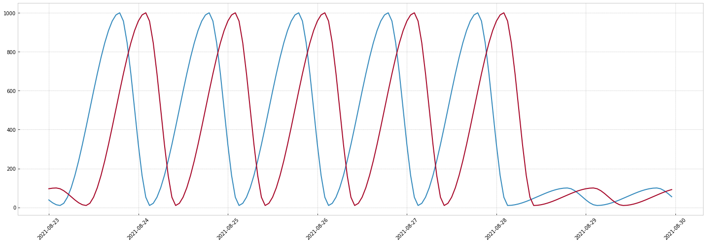
That's it! You can see the red curve corresponds to the PDT times.
Of course this also works with the other seasonalities presented in this tutorial.

Yearly seasonality - Normalizing

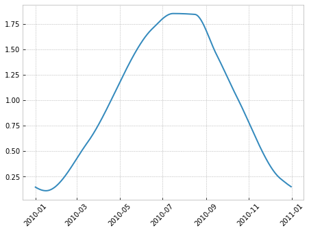
Let's have a look at the Historical monthly average temperature in Croatia from the World Bank Group.

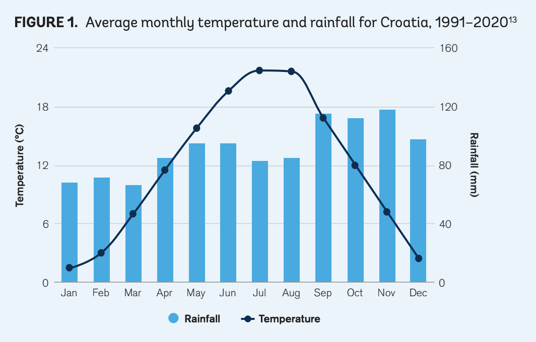
We have our pattern. It sounds reasonable to use the middle of a month to represent the average value of a month. For instance:

• January: timedelta(days=15)
• February: timedelta(days=46)
• October: timedelta(days=288).

Not easy to compute mentally, right ? Don't worry, middle-of-month timedeltas are available in the utils. Also, because we're lazy, we won't fill the 12 months and let the interpolation generate a realistic curve.

plt.rcParams["figure.figsize"] = DEFAULT_SIZE_PLOT

from mockseries.seasonality import YearlySeasonality

from mockseries.utils.timedeltas import JANUARY, MARCH, JUNE, JULY, AUGUST, SEPTEMBER, OCTOBER, DECEMBER

constraints = {

JANUARY: 1.3,

MARCH: 6.9,

JUNE: 20.1,

JULY: 21.9,

AUGUST: 21.8,

SEPTEMBER: 17.1,

OCTOBER: 12,

DECEMBER: 2.7,

}

yearly_seasonality = YearlySeasonality(constraints)

yearly_seasonality.preview_year(start_time=datetime(2021, 1, 1))

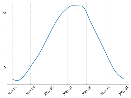
Repeating on multiple years:

import matplotlib.pyplot as plt

plt.rcParams["figure.figsize"] = LARGE_SIZE_PLOT

yearly_seasonality.preview_year(num_years=12, start_time=datetime(2010, 1, 1))

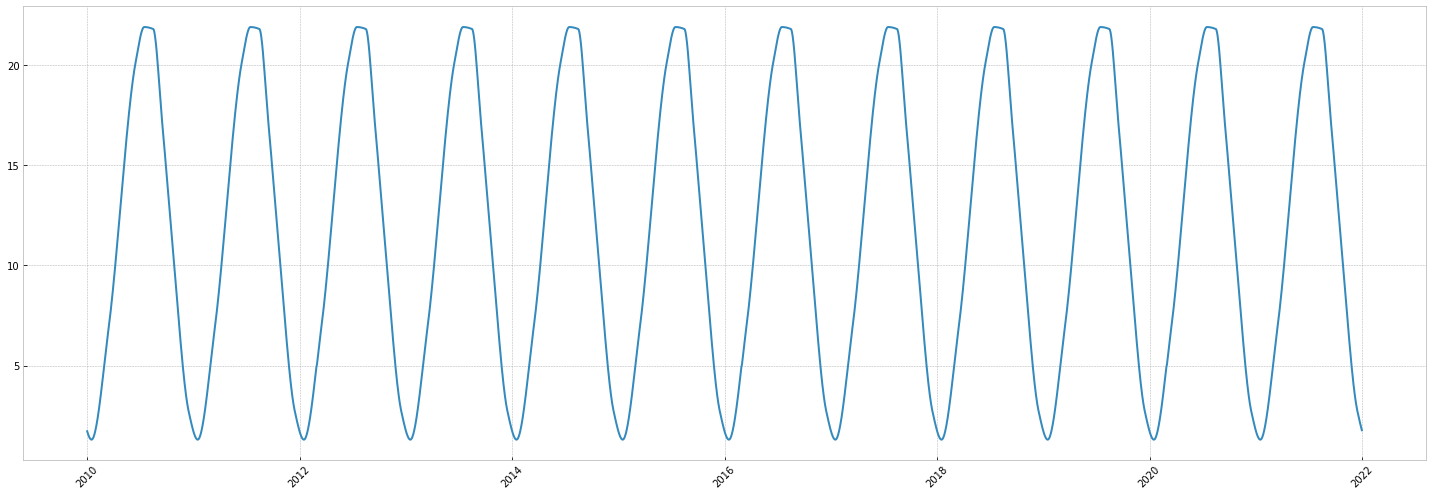
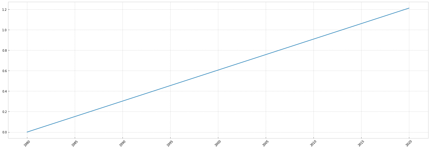
That's nice, but let's make this more realistic now. Look at the temperature trend: 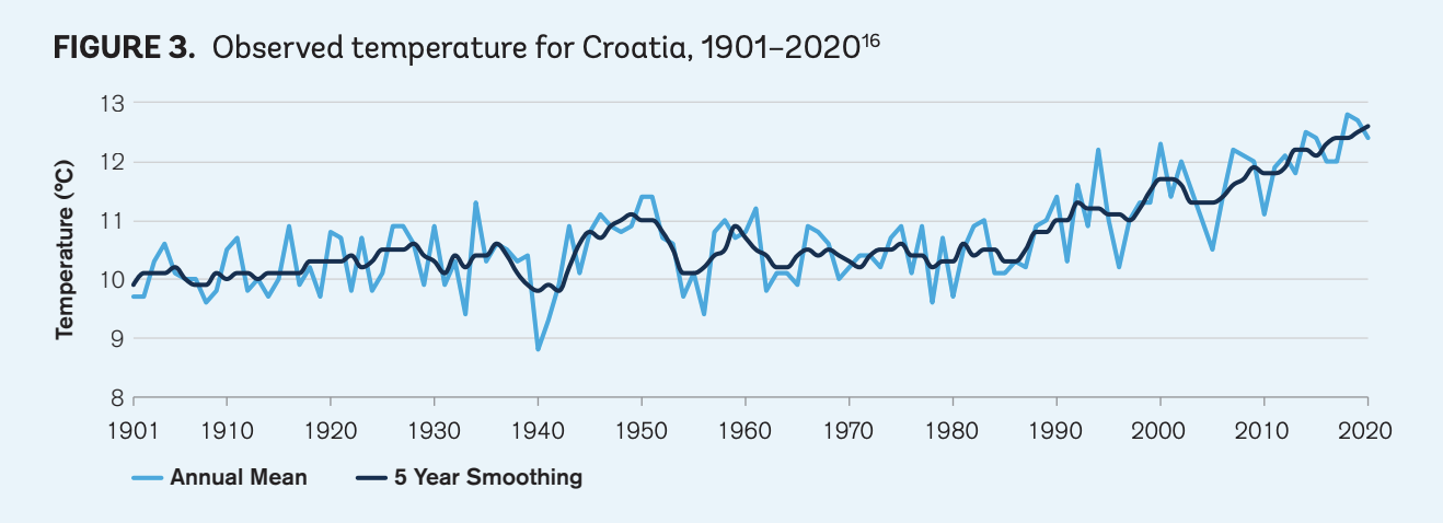In 1980 temperature averaged 10.4 degrees. It was 12.6 in 2020. We can roughly estimate that Croatia temperature follows a linear trend, raising by (12.6-10.4)/10.4 --> 21.1% in 40 years. Something like:

from mockseries.trend import LinearTrend

WARMING_COEFFICIENT = 1 + 0.211

PERIOD_YEARS = 40

trend = LinearTrend(coefficient=WARMING_COEFFICIENT,

time_unit=timedelta(days=365.25*PERIOD_YEARS),

)

# generate and plot

trend.preview_year(num_years=40, start_time=datetime(1980, 1, 1))

Let's combine this with our seasonality ! ... but how should we do this ? Our YearlySeasonality is based on average temperatures between 1990 and 2020. We would have to somehow estimate the true values in 1990, and then estimate the values in 1980. It's feasible with our linear trend approximation, but it's error prone.

Remember the two types of interactions ? A simple way to get around this is to use normalize in our YearlySeasonality. normalize transform constraints to a multiplication factor for easy use in multiplicative interactions. Let's check it out:

normalized_yearly_seasonality = YearlySeasonality(constraints, normalize=True)

plt.rcParams["figure.figsize"] = DEFAULT_SIZE_PLOT

normalized_yearly_seasonality.preview_year(start_time=datetime(2010, 1, 1))

Same curve, different scale.

Now it's easy to combine everything: we generate the base value, multiply it by our seasonality and add the trend. Also, let's add a bit of noise to make this more realistic.

from mockseries.noise import RedNoise

noise = RedNoise(0,1)

# combine signals - 10.4 is the value in 1980

timeseries = 10.4 * normalized_yearly_seasonality + trend + noise

# generate and plot for 20 years

plt.rcParams["figure.figsize"] = LARGE_SIZE_PLOT

timeseries.preview_year(num_years=50, start_time=datetime(1980, 1, 1))

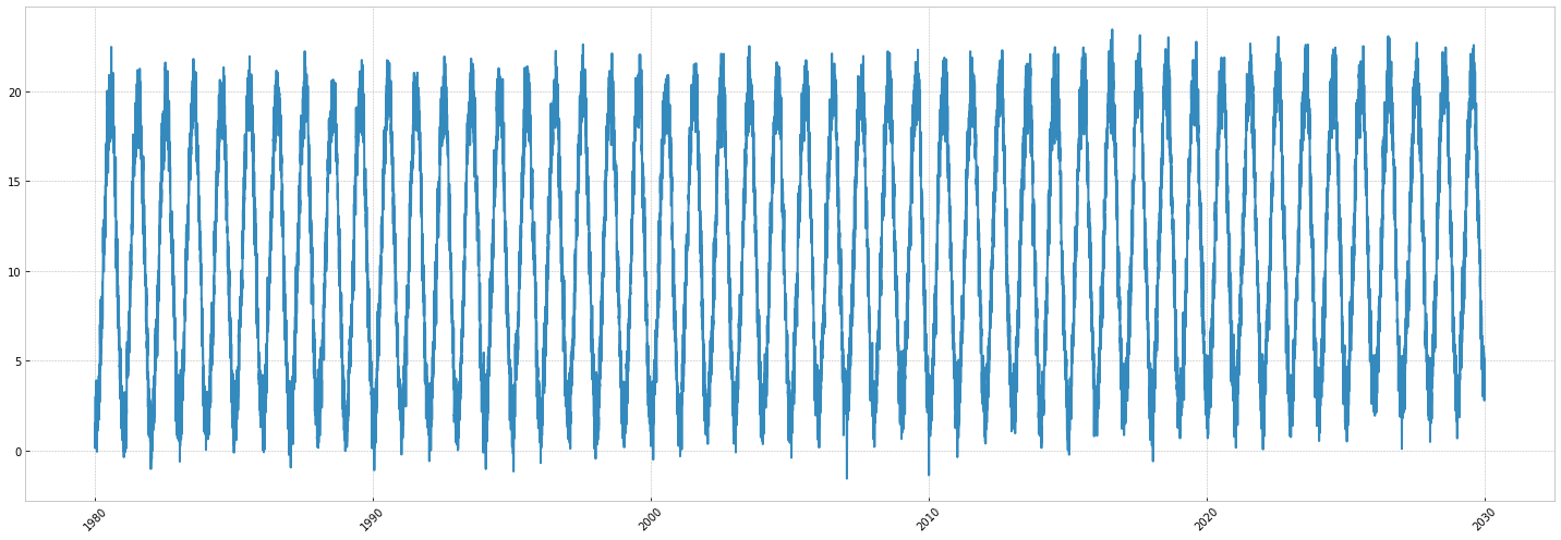
Here you are: a simple temperature timeseries for Croatia.
To go further, try to implement some improvements:

• Add the temperature's daily seasonality.
• Make the YearlySeasonality multiplicative with the trend.
• Make the trend non linear, exponential maybe.

Go to the next page to learn how to create switches, and point in time events.
Go directly to the PeriodSeasonality's API Reference to see how to extend the PeriodSeasonality for your own custom period.